ISSN 1884-0760
GRACE TECHNICAL REPORTS
Towards Bidirectional Transformations on Ordered
Graphs
Soichiro Hidaka
Kazuyuki Asada
Hiroyuki Kato
Keisuke Nakano
Zhenjiang Hu
GRACE-TR 2011–07 December 2011
CENTER FOR GLOBAL RESEARCH IN
ADVANCED SOFTWARE SCIENCE AND ENGINEERING NATIONAL INSTITUTE OF INFORMATICS 2-1-2 HITOTSUBASHI, CHIYODA-KU, TOKYO, JAPAN
1
Towards Bidirectional Transformations on Ordered Graphs
∗Soichiro Hidaka1, Kazuyuki Asada1, Hiroyuki Kato1, Keisuke Nakano2, and Zhenjiang Hu1
National Institute of Informatics1 University of Electro-Communications2
Abstract: The linguistic (language-based) approach plays an important role in de-velopment of structured and well-behaved bidirectional transformations. It has been successfully applied to solve the challenging problem of bidirectional transforma-tion on graphs, where a clear bidirectransforma-tional semantics is given based on a bulk se-mantics of the structural recursion. However, the graphs that can be dealt with are limited to unordered ones, and it has not yet been known how to treat ordered graphs such as XML graphs in which the child nodes of a node are ordered. In this paper, we show that the bulk semantics of structural recursion can be extended to ordered graphs, and that a clear bidirectional semantics of a new graph transformation lan-guage can be defined. The key technical point is a novel definition of bisimilarity between ordered graphs withε edges.
Keywords:Ordered Graphs, Graph Transformation, Bisimulation
1
Introduction
Bidirectional transformations [FGM+05,CFH+09] provide a novel mechanism for synchroniz-ing and maintainsynchroniz-ing the consistency of information between input and output. They are pervasive and have many potential applications, including the synchronization of replicated data in dif-ferent formats [FGM+05], presentation-oriented structured document development [HMT08], interactive user interface design [Mee98], coupled software transformation [L¨am04], and the well-knownview updatingmechanism which has been intensively studied in the database com-munity [BS81,Heg90].
The linguistic (language-based) approach [FGM+05] gives a promising way for development of structured and well-behaved bidirectional transformation, in which every expression simul-taneously specifies both a forward and the responding (correct) backward transformation, and every composite of expressions defines a structured way of gluing smaller bidirectional trans-formations to a bigger one. Despite its usefulness for bidirectional transtrans-formations on lists and trees [FGM+05,BFP+08,MHN+07,HMT08,Voi09,VHMW10,WGW11], it is a challenge to deal with bidirectional transformation on graphs. First, unlike lists and trees, there is no unique way of representing, constructing, or decomposing a general graph, and this requires a more precise definition of equivalencebetween two graphs. Second, graphs haveshared nodes and cycles, which makes both forward and backward computation more complicated than that on trees; na¨ıve computation would visit the same nodes many times and possibly infinitely.
∗ This is a full version of the paper submitted to the First International Workshop on Bidirectional Transformations
2 2 UNCALO: A TRANSFORMATION LANGUAGE FOR ORDERED GRAPHS
In our previous work [HHI+10], we challenged the problem by showing that the linguistic approach can be applied to bidirectional transformation on graphs, where a clear bidirectional semantics is given for UnCAL, a graph algebra for the known graph query language UnQL [BFS00]. The key to this success is the bulk semantics of the structural recursion: a structural recursion is evaluated by first processingin parallelall edges of the input graph and then com-bining the results. This bulk semantics relies on introduction ofε edges to graphs, providing a smart way of treating shared nodes and cycles in graphs and of tracing back from the view to the source.
However, the graphs that can be dealt with in this manner must be unordered. It has not yet been known how to treat ordered graphs such as XML graphs in which the child nodes of a node are ordered. One might consider encoding the ordered graphs in terms of unordered ones by introducing specialized edge labels, but this would make it difficult to keep consistency of these labels during transformation. In fact, it is an open problem, as pointed out in [BFS00], how to structure transformations on ordered graphs. In particular, it is unclear how to define a bulk semantics for transformations on ordered graphs.
In this paper, we show that the bulk semantics can be extended to ordered graphs, and that a clear bidirectional semantics of UnCALo, an ordered version of UnCAL, can be defined. The main technical contributions are three folds. First, we design a new graph transformation language UnCALo (Section2), which is similar to the graph algebra UnCAL [BFS00] for un-ordered graphs. Next, we give a novel definition of bisimulation relation on un-ordered graphs with
ε edges, propose the bulk semantics of structural recursion, and prove bisimulation genericity (well-definedness on bisimilarity) of the constructors and the structural recursion (Section 3). Finally, based on the above results, we show that the bidirectionalization method in [HHI+10] can be adapted to define bidirectional semantics of UnCALo(Section4).
2
UnCAL
o: A Transformation Language for Ordered Graphs
UnCALois a graph transformation language, which is similar to UnCAL [BFS00], but can dis-tinguish orders of outgoing edges. In UnCALo, we will use[] and++ for ordering instead of {}and∪used in UnCAL. The purpose of this section is to give an intuition of UnCALo. The formal definition of the semantics of UnCALois shown in Section3.
2.1 Graph Model
In UnCALo, graphs are rooted, directed, and edge-labeled graphs with order on outgoing edges. This graph data model has two prominent features,markersandε-edges. Nodes may be marked withinputandoutput markers, which are used as an interface to connect them to other graphs. Anε-edge represents a shortcut of two nodes, working like theε-transition in an automaton. We useL to denote the set of labels,Lε to denoteL ∪{ε},X to denote the set of input markers, andY to denote the set of output markers.
2.2 Graph Constructors 3
1
2
a
3
b
4
c
5
a a
c
6
d
(a) A Simple Graph
0
1
2 a
3 b
4 c
51 a 61
52 a
62
41 c 42
c
d d c
(b) An Equivalent Graph (c) Result ofa2d xcon (a)
Figure 1: Graph Equivalence Based on Bisimulation
node, which is calledinput node. Unlike input markers, more than one node can be marked with an identical output marker. They are calledoutput nodes. Intuitively, input nodes are root nodes of the graph (we allow a graph to have multiple root nodes, and for singly rooted graphs, we often use default marker&to indicate the root), while an output node can be seen as a “context-hole” of graphs where an input node with the same marker will be plugged in later.
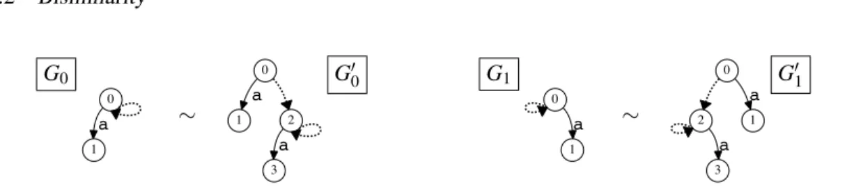
Note that multiple-marker graphs are meant to be an internal data structure for graph com-position. In fact, initial source graphs of our transformation have one input marker (single-rooted) and no output markers (no holes). For instance, the graph in Fig. 1(a) is denoted by (V,B,I)whereV={1,2,3,4,5,6},B(1) =[(a,2),(b,3),(c,4)],B(2) =[(a,5)],B(3) =[(a,5)], B(4) =[(c,4)],B(5) =[(d,6)],B(6) = [], andI(&) =1.
Notion of Graph Equivalence While a formal definition of graph equivalence will be given in Section 3, two graphs are value equivalent if they are bisimilar. For instance, the graph in Fig.1(b) is value equivalent to the graph in Fig.1(a); the new graph has an additional ε-edge (denoted by the dotted line), duplicates the graph rooted at node 5, and unfolds and splits the cy-cle at node 4. Unreachable parts are also disregarded, i.e., two bisimilar graphs are still bisimilar if one adds subgraphs unreachable from input nodes.
2.2 Graph Constructors
4 2 UNCALO: A TRANSFORMATION LANGUAGE FOR ORDERED GRAPHS
[] [a : G]
G a
G1 ++ G2
G1 G2 G
&z := G &z
&z ()
&x1 ... &xm
&y1 ... &yn
&x1’... &xm’
&y1 ... &yn
G1 G2
G1G2 G1@G2
&x1 ... &xm
&y1 ... &yn
G1
&z1 ... &zp
&y1 ... &yn
G2
ε ε
cycle(G)
&x1 ... &xm
&x1 ... &xm
ε ε
G &z
&x1 ... &xm
&y1 ... &yn
Figure 2: Graph Constructors
e ::= []|[l:e]|e++e|&x:=e|&y|()
| e⊕e|e@e|cycle(e) {constructor}
| $g {graph variable}
| let$g=eine { variable binding}
| ifl=ltheneelsee {conditional}
| rec(λ($l,$g).e)(e) {structural recursion application}
l ::= a|$l {label (a∈Lε) and label variable}
Figure 3: UnCALoLanguage
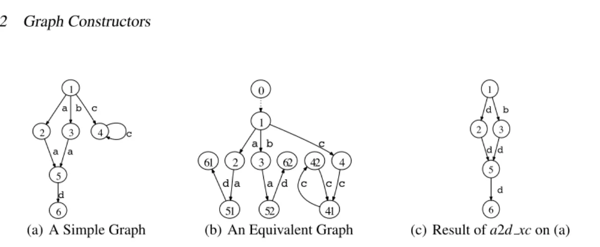
definition of the semantics of these constructors can be found in Section3. It is worth noting that this set of constructors are powerful enough to describe any ordered graph.
2.3 UnCALoSyntax
The syntax of UnCALois depicted in Fig. 3. As will be seen in Section3, UnCALo is bisim-ulation generic, i.e., for bisimilar inputs, each UnCALo expression results in bisimilar result. It consists of the graph constructors, variables1, variable bindings, conditionals, and structural recursion. We have already described the graph constructors, while variables, variable bindings and conditionals are self explanatory. Now we introducestructural recursion, which is a power-ful mechanism in UnCALoto describe graph transformations. A structural recursion is a function
f, which satisfies the following equations.
f([]) = []
f([$l: $g]) = e@f($g)
f($g1++$g2) = f($g1) ++f($g2),
5
and f can be encoded by rec(λ($l,$g).e). For[], f results in[]. For a graph with an edge labelled $l connected to a graph $g, f results in connecting vertically the result ofe with the result of recurring f to $g. For a graph with $g1 preceding $g2, f results in concatenating two graphs of f($g1)and f($g2).
Example1 The following structural recursiona2d xcreplaces all labelsawithdand contract
edges labeledc.
a2d xc($db) =rec(λ($l,$g).if $l=athen [d:&] else if $l=cthen[&]
else [$l:&]) ($db)
Applying the functiona2d xcto the graph in Fig.1(a)yields the graph in Fig.1(c).
Example2 Consider an ordered graph representation of books. Since “sections” are ordered and there are some references in books, we can see books as ordered graphs. The following structural recursion toc, which is adapted from [RSGV09], computes the table of contents of books in which sections can be arbitrarily nested:
toc($db) =rec(λ($l,$g).if $l=sectionthen[section: [gettitle($g),&]] else &) ($db)
where the functiongettitleresults in the title of the section.
gettitle($g) =rec(λ($l1,$g1).if$l1=titlethen[title:rec(λ($l2,$g1).[$l2: []]) ($g1)]
else []) ($g)
3
Ordered Graph and Structural Recursion
In the previous section, we gave syntax of UnCALo, its intuitive meaning, and its usage. In this section, we give semantics of UnCALo. In the next section, we extend the semantics here for bidirectional transformation, where ε-edge and bulk semantics for structural recursion— main contents in this section—are importantly used to keep source information during forward transformation. Thus we heavily useε-edge, so the bisimilarity for ordered graph withε-edges is important.
Here we first give definitions of ordered graph and its bisimilarity. These ordered graphs up to bisimilarity form the domain of the semantics of UnCALo. Next we define graph con-structors and structural recursion with bulk semantics. Then we showbisimulation genericity
(well-definedness on bisimilarity) of the graph constructors and the structural recursion (Theo-rem1).
6 3 ORDERED GRAPH AND STRUCTURAL RECURSION
3.1 Formal Definition of Ordered Graph
Definition 1 (Ordered Graph) LetL be a set oflabels, andLε be the disjoint unionL ∪{ε}. LetXbe a finite set ofinput markersandY be a finite set ofoutput markers.
Anordered graph, or just agraph Gis a triple(V,B,I)where • V is a set ofnodes,
• B:V → ∏ n∈N(Lε×V+Y)n is a function, which maps a node to its ordered branches
consisting oflabeled edgesoroutput markers, and
• I:X→V is a function, which determinesroots (input nodes)of the graph.
The set of all graphs (defined withX andY) is denoted byDBXY (meaning DataBase follow-ing [BFS00]). For a graphG, we refer to each component of the triple by record notation with labels V,B,I: i.e.,G= (G.V,G.B,G.I).
Remark1 In the paper [BFS00], unordered graph was defined additionally with the following three requirements: an input functionI is injective; there is no incoming edge to an input node; and there is no outgoing edge from an output node. While, the above definition of ordered graph is relaxed on such points. The both styles are in fact equivalent: i.e., for the above style of a graph, if we extend each input node with a fresh epsilon edge incoming from a fresh new input node, and also replace each output marker occurrence on an output node by a fresh epsilon edge outgoing to a fresh node having only the branch of the output marker, then the resulting graph satisfies the above three requirements, and still is bisimilar (Definition5) to the given graph. This transformation is possible for both unordered case and ordered case.
As meta-variables for markers, we use&x,&y,&z, etc. Since we often consider single-rooted graphs, i.e., graphs whose sets of input markers are singleton, we choose adefault marker de-noted by&, andDB{&}
Y is denoted byDBY.
In the above definition, ∏ n∈N(Lε×V+Y)n=List(Lε×V+Y). To represent ordered branch,
“list in polynomial style” is more essential than “list as initial algebra”, since with polynomial style, the more generalized notion ofgraph with countably wide ordered branchcan be similarly defined withB:V → ∏ L∈L(Lε×V+Y)LwhereLis the set of countable linear ordered sets (up
to order isomorphism).
For a listx,|x|denotes the length ofx, and we regard|x|also as the set of component-indices ofx, i.e., |x|={0, ...,|x|−1}. Then fori∈|x|, x.idenotes thei-th component of x. We often represent a list as[xi]i∈n, as well as an extensional style such as [x,y,z]. For a tuple x∈∏i∈IXi
and an indexi∈I, we usex.ito denote thei-th component ofx: e.g., forx∈A×B,x= (x.0,x.1). For setsA andB, an element of the coproductA+B is either inl(a) witha∈Aexclusively or
inr(b)withb∈B. For ternary coproduct, we use inl, inm, and inr.
For a graphG= (V,B,I), a nodev∈V, and a branch indexi∈|B(v)|, the list componentB(v).i
3.2 Bisimilarity 7
G0
0
1
a ∼
0
2 1
a
3
a
G′0 G1
0
1
a ∼
0
2 1
a
3
a
G′1
Figure 4: graphs with left-to-right-stream branching and with right-to-left-stream branching
For a graphG, we callG finiteifG.V is finite. In this section, we also consider infinite graphs because we need infinite graph (in fact infinite tree) to define bisimilarity even for finite graph. In other sections, we treat only finite graphs and call them just (ordered) graphs.
For a graphG∈DBYX, and a nodev∈G.V, G|v denotes the graph inDBY whose set of nodes
are restricted to the set of all nodes “accessible through consecutive branches” fromv.
For a graphG∈DBXY,Gis atreeif (i): G.I is injective, (ii): for every root node, there is no incoming edge, (iii): for every non-root nodes, there is exactly one incoming edge, and (iv) any node can be accessible from a root node in finite steps. (For finite graphs, the condition (iv) is derived from the conditions (ii) and (iii).) The conditions (ii) and (iii) keep out cycle and sharing from tree. Note that ift is a tree, so ist|v for anyv∈t.V, and also that any multi-rooted tree t∈DBXY is the disjoint union of the family(t|t.I(&x)))&x∈X of the single-rooted trees.
3.2 Bisimilarity
Bisimilarity between ordered graph is—if the notion does not involveε-edge—easily defined with a general coalgebraic definition (e.g. [Rut00, SR11]) applied to the endofunctor V *→ List(L ×V+Y). However, for ordered graph withε-edges, the definition of bisimilarity is not obvious. In the unordered case, we can take the approach in the paper [BJ10], but for ordered case, it is not available.
First let us see the bisimilarity for the case withoutε-edge.
Definition 2 For ordered graphs G,G′ ∈DBYX withoutε-edges,G andG′ are bisimilar(and denoted by G∼L G′) if there is a relation R betweenG.V and G′.V such that (i): for every input marker&x∈X, (G.I(&x))R(G′.I(&x)), and (ii): R is abisimulation relation: i.e., for any
vRv′,|G.B(v)|=|G′.B(v′)|, and then for anyi∈|G.B(v)|, either if(G.B(v)).i=E(l,v1), then there isv′1∈G′.V such that(G′.B(v′)).i=E(l,v′1) andv1Rv′1, or if(G.B(v)).i=O(&y), then (G′.B(v)).i=O(&y).
Now let us see some ordered graphs withε-edges, to have some feeling of bisimilarity. Con-sider graphs in Figure 4. The graphs Gi should be intuitively bisimilar respectively to their
1-step-unfoldingG′i, because unfolding generally maintains bisimilarity. Here, we should distin-guishG0fromG1. This is because, observing their further unfolding, it is found thatG0is a tree with height one and with countable width of branch, and the order of the branching is like an infinite stream from left to right; on the other hand, the graphG1is similar one but the branch is like an infinite stream from right to left.
8 3 ORDERED GRAPH AND STRUCTURAL RECURSION
|G′.B(v)|” above; on this point for the case with ε-edge, we first extend the notion of list of branches to that of linear ordered set of branches, and then compare them in terms of order isomorphism. For the examples,G0 has no maximum (right side) but has minimum (left side), whileG1has maximum and has no minimum, so they are not isomorphic, and hence not bisim-ilar. (Order isomorphism was implicit in the case withoutε-edge, since for finite linear ordered sets, to be order isomorphic is determined just by their cardinalities.) In order to define sets of all such branches and to define linear orders on them, we first unfold graphs to trees.
Thus we define bisimilarity for ordered graph withε-edges in two steps: we first unfold graphs to trees, which might be infinite even for finite graphs; and then determine “proper” branches by taking transitive closure ofε-edges, and “bi-simulate” them with order isomorphisms.
The definition of unfolding of graph to tree is usual one, which keepsε-edges, regardingε as a normal label inL.
Definition 3 (Unfolding) LetG= (V,B,I)∈DBYX. We define a tree uf(G)∈DBXY as in the following.
We will define only for the case thatXis a singleton, say{&}, then for the other case, we can define uf(G)as the disjoint union tree of family(uf(G|(G.I)(&x)))&x∈X of single-rooted graphs.
First we define a family of disjoint sets (Vn)n∈N by induction on n∈N, asVn will be the set of n-depth nodesv∈uf(G).V, and there v= (the depth n of v, the parent node ofv, the corresponding node in the original graphG, the branch index ofv).
• V0 def
={(0,⊥,I(&),⊥)}, where the element will be the root, hence⊥in the two undefinable components is just some dummy.
• Vn+1 def
={(n+1,x,v,i) | x∈Vn, i∈|B(x.2)|, B(x.2).i=inl(l,v)}
Then uf(G)def= (!
n∈NVn,B′,{&*→(0,⊥,I(&),⊥)})∈DBY where forx∈Vn,
B′(x)def=
"
B(x.2).i=E(l,v) ⇒ E(l,(n+1,x,v,i)) =O(&y) ⇒ O(&y)
#
i∈|B(x.2)|
For graphs G and G′ (possibly with ε-edges), we can define their bisimilarity observing ε
(denoted byG∼!G′) just asG∼Lε G′, where we regardε as a normal label. Then it is easily shown thatG∼!G′if and only if uf(G)and uf(G′)are (uniquely) isomorphic. We use this notion of bisimilarity observingεin the proof of bisimulation genericity (Theorem1).
Now let us go to the second step; first we consider transitive closure ofε-edges.
For a treeT ∈DBYX and a nodev∈T.V, letv0be aself-or-ancestor ofv, i.e., there is a path
v0
l0
→i0 ...vn−1 ln−1 →in−1 vn(
def
=v)(n∈N)wherevj lj
→ij vj+1meansG.B(vj).ij =E(lj,vj+1). Note
that by the condition of tree, such path is unique. Then for a branch indexi∈|T.B(v)|ofv, the pair(v,i)isproper branch of v0if (i): alllj areε, and (ii): ifT.B(v).i=E(l,v′)for someland v′, thenl-=ε. (Note that for the case thatT.B(v).i=O(&y), the condition (ii) holds.) For a tree
T ∈DBYX and a nodev0∈T.V, Pb(T,v0)denotes the set of all proper branches ofv0.
Then there is a natural linear order ≤Pb on Pb(T,v0): for two different proper branches (v,i) and(v′,i′), we compare the two branches of the lowest one—in terms of depth of tree— among common self-or-ancestors ofv and v′. Formally, letv0→ε i0 ...vn−1
ε
→in−1 vn(
3.3 Graph Constructors and Bulk Semantics for Structural Recursion 9
v′0(def=v0)→ε i′
0 ...v
′
n′−1
ε
→i′
n′−1v
′
n′(
def
=v′)be respectively the paths fromv0tovandv′; and also let
in
def
=iandi′n′
def
=i′. Then by conditions in the definition of proper branch,(vmin(n,n′),imin(n,n′))-=
(v′min(n,n′),i′min(n,n′)), hence we can take the leastksuch that(vk,ik)-= (v′k,i′k)ask0. Then we can show thatvk0 =v
′
k0, henceik0 -=i
′
k0. Now we define as(v,i)<Pb(v
′,i′)⇐⇒def i
k0<i
′
k0.
Now let us go to the second step for defining bisimilarity of ordered graph.
Definition 4 (Bisimilarity for Tree) For a pair of treesT,T′∈DBYX,T andT′ arebisimilar if there is a relationRbetweenT.V andT′.V such that
• for every input marker&x∈X, (T.I(&x))R(T′.I(&x)), and
• R is a bisimulation relation: i.e., for any v0Rv′0, there is an order isomorphism f : (Pb(T,v0),≤Pb)→(Pb(T′,v′0),≤Pb) satisfying the following property. For any proper branch(v,i)∈Pb(T,v0), let(v′,i′)be f(v,i). Then,
– for anyl∈L,u∈T.V, ifT.B(v).i=E(l, u), then there existu′such thatT′.B(v′).i′= E(l, u′)anduRu′, and
– for any&y∈Y, ifT.B(v).i=O(&y), thenT′.B(v′).i′=O(&y).
It can be checked that the above bisimilarity relation is symmetric and an equivalence relation.
Definition 5 (Bisimilarity for Ordered Graph with ε-edges) For graphs G,G′∈DBYX, Gand
G′ are bisimilar (and denoted by G∼G′) if uf(G) and uf(G′) are bisimilar (in the sense of Definition4). (Bisimilarity is calledvalue equivalencein [BFS00].)
For a treeT ∈DBXY,T and uf(T)are equal up to the unique isomorphism. Hence for any pair of trees, the two bisimilarity above are equivalent, and not ambiguous.
For a pair of graphsG,G′∈DBXY, ifGandG′ has noε-edge, thenG∼G′⇐⇒G∼!G′⇐⇒
G∼LG′. Otherwise, ifG∼!G′thenG∼G′, but the converse is not necessarily true.
3.3 Graph Constructors and Bulk Semantics for Structural Recursion
Now we define graph constructors and a structural recursion; we use the same function name as the name of a function symbol in the syntax.
Definition 6 (Graph Constructors)
• []def= ({&},{&*→[]},id{&})∈DBY
• ForG∈DBY, [l:G]
def
= (G.V∪{v0: fresh},G.B∪{v0*→[E(l,G.I(&))]},{&*→v0})∈DBY
• ForGl∈DBXY andGr∈DBYX, Gl++Gr
def
= (Gl.V+X+Gr.V,B′,inm)∈DBXY where
B′(ink(v))
def =
(k=lorr) "
Gk.B(v).i=E
$
l, v′% ⇒ E$
l,ink(v′)
%
=O(&y) ⇒ O(&y)
#
i∈|gk.B(v)|
B′(inm(&x))
def
10 3 ORDERED GRAPH AND STRUCTURAL RECURSION
• ForG∈DBY, (&x:=G)
def
= (G.V,G.B,{&x*→G.I(&)})∈DB{&x}
Y
• For&y∈Y,&ydef= ({&},{&*→[O(&y)]},id{&})∈DBY
• ()def= (/0,/0,id/0)∈DBY/0
• For Gl ∈DBYXl andGr∈DBYXr such thatXl∩Xr= /0, Gl⊕Gr
def
= (Gl.V+Gr.V,B′,I′)∈ DBXl∪Xr
Y where
B′(ink(v))
def =
(k=lorr) "
Gk.B(v).i=E
$
l, v′% ⇒ E$l,ink(v′)%
=O(&y) ⇒ O(&y)
#
i∈|Gk.B(v)| I′(&x)def= inl(Gl.I(&x)) (if&x∈Xl) or inr(Gr.I(&x)) (if&x∈Xr) • ForGl∈DBXY andGr∈DBYZ, Gl@Gr
def
= (Gl.V+Gr.V,B′,inl◦Gl.I)∈DBXZ where
B′(ink(v))
def =
(k=lorr)
Gk.B(v).i=E
$
l,v′%
⇒ E$
l,ink(v′)
%
=O(&w) ⇒
)
k=l ⇒ E(ε,inr(Gr.I(&w)))
=r ⇒ O(&w)
i∈|gk.B(v)|
• ForG∈DBXX∪Y such thatX∩Y =/0, cycle(G)def= (G.V,B′,G.I)∈DBXY where
B′(v)def=
"
B(v).i=E$
l, v′%
orO(&y) (&y∈Y) ⇒ B(v).i
=O(&x) (&x∈X) ⇒ E(ε, G.I(&x))
#
i∈|B(v)|
Remark2 The definition ofcycleabove is different from that in the paper [BFS00]: i.e., we just added cycling epsilon edges, while in loc. cit. additionally each input node is extended with a fresh epsilon edge incoming from a fresh new input node. This is just (a part of) the transformation in Remark1and hence the both are equivalent.
Definition 7 (Bulk Semantics of Structural Recursion) Fore:L ×DBY →DBZ
Z, astructural recursion function (for ordered graph)rec(e):DBXY →DBZZ××YX is defined as the following.
Let G= (V,B,I)∈DBYX. We extend e to ¯e:Lε×DBY →DBZ
Z which maps (ε, ) to the
“identity” graph(Z,{&z*→[O(&z)]},idZ). For a listx∈List(Lε×V+Y), letx|edgedef={(i,l,v)∈ N×Lε×V |i∈|x|,x.i=E(l,v)}.
Thenrec(e)(G)def= (V′,B′,I′)where • V′def= (Z×V) + ( ∏ v∈V,(i,l,v′)∈B(v)|
edgee¯(l,G|v′).V)
(We simplify the indices in ∏ v∈V,(i,l,v′)∈B(v)|
edge just as ∏
v,i,l,v′, in the following.)
• B′:(Z×V)+( ∏ v,i,l,v′e¯(l,G|v′).V)→ ∏ n
-Lε×$
(Z×V)+( ∏ v,i,l,v′e¯(l,G|v′).V)%+Z×Y .n
inl(&z,v) *→
"
B(v).i=E$l, v′% ⇒ E$ε,inr$
(v,i,l,v′),e¯(l,G|v′).I(&z)%% =O(&y) ⇒ O((&z,&y))
#
i∈|B(v)|
inr((v,i,l,v′),u) *→
(xdef= (e¯(l,G|v′).B)(u)) "
x.i=E$
l′, u′%⇒ E$
l′,inr
$
(v,i,l,v′),u′%%
=O(&z) ⇒ E$ε,inl(&z,v′)%
#
3.3 Graph Constructors and Bulk Semantics for Structural Recursion 11
• I′: Z×X → (Z×V) + ( ∏ v,i,l,v′e¯(l,G|v′).V): (&z,&x)*→inl(&z,I(&x))
It should be noticed that the above graph constructors are closed on finiteness, i.e., they map finite graphs to a finite graph; and also ifeis closed on finiteness, so isrec(e).
From now we show that the above functions on graphs are bisimulation generic.
Definition 8 (Bisimulation Genericities) Let f :DBX1
Y1 ×...×DB Xn Yn →DB
X
Y. Then f is bisim-ulation generic if for G1∼G′1, ...,Gn ∼G′n, f(G1, ...,Gn) ∼ f(G1′, ...,G′n); and f is strongly bisimulation genericif both f isbisimulation generic observingε, i.e., forG1∼!G′1, ...,Gn∼!
G′n, f(G1, ...,Gn)∼! f(G′1, ...,G′n), and f is bisimulation generic for trees, i.e., for trees T1 ∼
T1′, ...,Tn∼Tn′, f(T1, ...,Tn)∼f(T1′, ...,Tn′).
Since our bisimilarity was defined in two steps, proving bisimulation genericity is compli-cated, so we split the bisimulation genericity into the two simpler bisimulation genericities:
Lemma 1 Let f :DBX1
Y1 ×...×DB Xn Yn →DB
X
Y. If f is strongly bisimulation generic, then f is bisimulation generic.
Proof. Let f :DBYX →DBYX′′ be a unary function to keep presentation simple, and assume the
both assumption in the statement andG∼G′. Our goal is to prove that f(G)∼f(G′).
By the definition of the bisimilarity, G∼G′ implies uf(G)∼uf(G′). Now f is bisimulation generic for trees uf(G) and uf(G′), so f(uf(G))∼ f(uf(G′)). On the other hand, since f is bisimulation generic observingε, and sinceG∼!uf(G)andG′∼!uf(G′), it holds that f(G)∼!
f(uf(G)) and f(G′)∼! f(uf(G′)). Since∼! implies ∼, hence f(G)∼ f(uf(G)) and f(G′)∼
f(uf(G′)). Thus it is derived that f(G)∼ f(G′).
We remark that the converse of this lemma is trivially false. Because, take such graphsG0,G1,
andG′0thatG0∼G1, notG0∼!G1,G0∼!G′0, andG0=- G′0. Then we define f(G) def
=ifG=G0 then G1 else G. Then, since f(G)∼G, f is bisimulation generic; but f is not bisimulation generic observingε, sinceG0∼!G′0and not f(G0)∼!f(G′0).
Theorem 1 The graph constructors and the structural recursion are strongly bisimulation generic. The latter means that for e:L ×DBY →DBZ
Z, if for any l ∈L, e(l,-) is strongly bisimulation generic, then so isrec(e):DBYX →DBZZ××YX.
Proof. We omit similar parts to the proof of the similar theorem in the paper [BFS00], and describe other points proper to this ordered case. On the case of graph constructors, the proofs are straightforward. For the structural recursion, first we can directly show that ifeis bisimulation generic observing ε, then so is rec(e). We can also directly show that for any graph g and
e,e′:L ×DBY →DBZ
Z, ife∼!e′(pointwisely), thenrec(e)(G)∼!rec(e′)(G). Then using this,
12 4 BIDIRECTIONAL SEMANTICS OF ORDERED UNCAL
4
Bidirectional semantics of Ordered UnCAL
In this section, we provide bidirectional semantics for UnCALoproposed in Section2, enriching the semantics given in Section3. We adapt our previous work [HHI+10] on unordeded UnCAL. The overall framework in the previous work—enriching forward semantics by trace information, and providing backward semantics for the forward transformation—remains unchanged. In par-ticular, we decompose target graphs in the backward transformation based on operators having produced the trace information, and produce updated variable binding environment as a result of backward transformation. As in the forward semantics, the order between the branches of each node is respected in the backward transformation. The major difference between the bidirec-tional semantics of unordered UnCAL and that of UnCALois that branches are represented as ordered lists instead of sets. However, the fact that the union operator is no longer commutative does not essentially change the backward evaluation. For example, when we unify the result of binary operation, the order between the operands are not reflected.
Bidirectional Properties Our goal in bidirectionalizing UnCALois to have bidirectional prop-erties inherited from the previous work [HHI+10]. LetF[[e]]ρ denote a forward evaluation (get) of expression e under environmentρ to produce a view, and B[[e]](ρ,G′) denote a backward
evaluation (put) of expressione under environmentρ to reflect a possibly modified viewG′ to the source by computing an updated environment. Anenvironmentρ is a mapping with a form of{$x*→X, . . .}whereX is a graphGor a labell. The following are two properties we aim at:
F[[e]]ρ=G
B[[e]](ρ,G) =ρ(GETPUT)
B[[e]](ρ,G′) =ρ′ F[[e]]ρ′=G′′
B[[e]](ρ,G′′) =ρ′ (WPUTGET)
The(GETPUT)property states that unchanged viewGshould give no change on the environment
ρ in the backward evaluation, while the(WPUTGET)property states that the modified viewG′
and the view obtained by backward evaluation followed by forward evaluation may differ, but both views have the same effect on the original source if backward evaluation is applied. A pair of forward and backward evaluations iswell-behavedif it satisfies(GETPUT)and(WPUTGET)
properties. In the rest of this paper, we will present forward and backward evaluations (bidirec-tional semantics) for UnCALoand prove the following theorem.
Theorem 2 (Well-behavedness) The proposed forward and backward evaluations are well-behaved, provided their evaluations succeed.
In the rest of this section, we first provide forward semantics enriched with trace information, and then define backward semantics using the trace information.
4.1 Traceable Forward Evaluation
4.2 Enriched Forward Semantics 13
trace IDis defined by
TraceID::=SrcID|CodePos Marker
| RecNPos TraceID Marker|RecEPos TraceID TraceID Num,
whereSrcID ranges over identifiers uniquely assigned to all nodes of the database,Posranges over code positions in the UnCALo expression,Markerranges over input/output markers, and
Numstands for integers. This trace ID is different from that of the previous work in that in the RecE part,TraceID and ordinalNum is used instead of edge. The Numpart represents from which branch of the input graph ofrecthe node is produced. In unordered setting, the position in the set of branches are not important, so the edge, i.e, triple of source node, label and target node was sufficient. In ordered setting, he have to keep track of the position. For example, if a nodewis generated from thei-th branch(l,vt)of nodevsthrough therecconstruct at the code
positionp, then trace ID of the formRecEw vsiis produced.
4.2 Enriched Forward Semantics
We now formally define the enriched forward semantics for finite graphs by simple augmenta-tion of trace IDs to the semantics in the previous secaugmenta-tion. We still use(V,B,I) representation, but we use TraceID structure for nodes inV instead of products and coproducts. In addition, we replace the composition of markers inX×Z by a monoid(·,&), with&as the identity, i.e., &·&x=&x·&=&x. The type ofrecwill be(L×DBY→DBZZ)→DBYX→DBZ·X
Z·Y, whereZ·X is
defined by{&z·&x|&z∈Z,&x∈X}. In particular,{&} ·Z=Z· {&}=Zfor anyZ. This treatment is inherited from [BFS00], and easier to implement. It is not for the sake of bidirectionalization. For example,rec(λ($l,$t).e)(G)∈DBYX fore:(L×DBY →DB&)andG∈DBX
Y, meaning that
a recwith the body that consists only of the default marker does not change the type of their input graphs through applications. So++inrec(λ($l,$t).e)(G) ++Gis well defined (recall that operands of++must have identical set of input markers). In order for the newrecto be well-defined, however, we should restrict the combination ofZ andX so thatZ·X is isomorphic to
Z×X. For example, if bothZ andX include the default marker&and a non-default marker in common, then I component in the result ofrecis ill-defined, mapping identical input marker to more than one nodes. In practice, Z either contains only the default marker, or contains only non-default markers. In the following definitions, ep denotes an UnCALo subexpression e at code position p,ρ($x)denotesGwhen($x*→G)∈ρ. ρis naturally used as variable substitu-tion in UnCALoexpressions, e.g.,eρfor an expressione. As in [HHI+10], we inductively define the enriched forward semanticsF[[ep]]ρfor each UnCALoconstruct ofe.
Graph Constructor Expressions.The semantics of graph constructor expressions is a straight-forward extension of that in section3. For instance, we have
F[[
p
[]]]ρ= ({Codep},{Codep*→[]},{&*→Codep}),
14 4 BIDIRECTIONAL SEMANTICS OF ORDERED UNCAL
As another example, the semantics for the expressione1++e2is defined below.
F[[(e1++e2)p]]ρ =F[[e
1]]ρ++pF[[e2]]ρ G1++pG2= (V∪G1.V∪G2.V,B∪G1.B∪G2.B,I) where M=inMarker(G1) =inMarker(G2) V ={Codep&m|&m∈M}
B={Codep&m*→[E(ε,I1(&m)),E(ε, I2(&m))]|&m∈M}
I ={&m*→Codep&m|&m∈M},
where++pis a union operator for two graphs concerning position p. We writeinMarker(G)to
denote the set of input markers andoutMarker(G)to denote the set of output markers in a graph
G.
e1⊕e2It performs a componentwise union like++, except that noε-edges are involved.
F[[(e1⊕e2)p]]ρ =F[[e1]]ρ⊕F[[e2]]ρ,
where⊕is a componentwise union operator for two graphs. A graphG1⊕G2is defined by
G1⊕G2 = (V1∪V2,B1∪B2,I1∪I2) where (V1,B1,I1) =G1
(V2,B2,I2) =G2
inMarker(G1)∩inMarker(G2) = /0
Nullary constructors&yand ()These expressions construct constant graphs: &y constructs a node with a default input marker&and an output marker&y, and()constructs the empty graph.
F[[&mp]]ρ = ({Codep},{Codep*→[O(&m)]},{&*→Codep}) F[[()p]]ρ = (/0,/0,/0)
[l:e]
F[[[l:e]p]]ρ =
({Codep}∪V,{Codep*→[(lρ,I(&))]}∪B,{&*→Codep}) where (V,B,I) =F[[e]]ρ
Trace IDCodeis generated for the newly constructed node.
e1@e2It appends two graphs by connecting the output nodes of the left operand and correspond-ing input nodes of the right operand withε-edges.
F[[(e1@e2)p]]ρ =F[[e1]]ρ@pF[[e2]]ρ,
where@p is an append operator for two graphs concerning position p. A graph G1@pG2 is defined by
G1@pG2 = (G1.V∪G2.V,B′1∪G2.B,G1.I)
where B′1 =
)
u*→
/
x.i= (l,v) ⇒ (l,v)
=&m ⇒ (ε,G2.I(&m))
0
i∈|x|
|(u*→x)∈G1.B
4.2 Enriched Forward Semantics 15
Note that@may introduce unreachable parts in the right operand due to unmatched input/output nodes.
&m:=eIt distributes the marker on the left operand to each of the input markers of the graph in the right operand, using the Skolem function “.” introduced at the beginning of this section.
F[[(&m:=e)p]]ρ = (&m:=F[[e]]ρ),
where :=is an operator for a marker distribution for a graph. A graph(&m:=G)is defined by
(&m:=G) = (V,E,I′) where (V,E,I,O) =G
I′ ={&m.&x*→v|(&x*→v)∈I}
cycle(e)It is defined as follows
F[[(cycle(e))p]]ρ =cyclep(F[[e]]ρ) cyclep(G) = (G.V,B′,G.I)
where B′(u) =
G.B(u).i=E(l, v) ⇒ E(l, v) =O(&m)∧&m∈dom(I) ⇒ E(ε,I(&m)) =O(&m)∧&m∈/dom(I) ⇒ O(&m)
i∈|G.B(u)|
wherecyclepis a cycle operator for a graph concerning positionp.
Variable and Condition.They have the following obvious definitions.
F[[($v)p]]ρ=ρ($v) F[[(ifl
1=l2thene1elsee2)p]]ρ=
2
F[[e1]]ρ ifl1ρ=l2ρ F[[e2]]ρ otherwise.
rec(λ($l,$g).eb)(ea)The semantics of a structural recursion is given by bulk semanticsas de-fined in Section3. Following [HHI+10], we define the enriched forward semantics of structural recursion by two auxiliary functionscomposerecandfwd eachedge:
F[[(rec(λ($l,$g).eb)(ea))p]]ρ = composep
rec(fwd eachedge(Ga,ρ,eb),Ga,M) where M =inMarker(eb)∪outMarker(eb)
Ga =F[[ea]]ρ
16 4 BIDIRECTIONAL SEMANTICS OF ORDERED UNCAL
fwd eachedge(G,ρ,e) = {(v,i,vi,F[[e¯]]ρv,i)
| v∈G.V,x∈G.B(v), i∈|x|,E(li,vi) =x.i, ρv,i=ρ∪{$l*→li,$g*→G|v}} composerecp (G,G,M) = (VRecE∪VRecN,BRecE∪BRecN,IRecN)
whereVRecE ={RecE p w v i | (v,i, ,Gv,i)∈G,w∈Gv,i.V}
BRecE = 2
RecEp w v i*→
/
x.j=E(lj,wj) ⇒ E(lj, RecEp wjv i)
=O(&m) ⇒ E(ε, RecNp vi&m)
0
j∈|x| | (v,i,vi,Gv,i)∈G,w∈Gv,i.V,x=Gv,i.B(w)}
VRecN ={RecNp v&m | v∈G.V, &m∈M} BRecN ={RecNp v&m*→
/
x.i=E(li,vi) ⇒ E(ε, RecEp Gv,i.I(&m)v i) where(v,i, ,Gv,i)∈G
=O(&n) ⇒ O(&m·&n)
0
i∈|x| | v∈G.V,x=G.B(v),&m∈M}
IRecN ={&n·&m*→RecNp v&m | G.I(&n) =v,&m∈M}
4.3 Backward Semantics
Thanks to the bulk semantics defined in Section3and trace information generated at enriched forward evaluation, the similarity in shape between input and output graphs are retained. As in the previous work [HHI+10], the graph constructors become invertible, and backward evaluation ofrec(e) is reduced to that of its bodye. We again divide backward evaluation algorithm by updates supported: (1) edge-renaming, (2) edge-deletion, and (3) insertion of edges or a subgraph rooted at a node. In the following, we give the backward semantics for these updates.
4.3.1 Backward Semantics for Edge Renaming
Backward semantics is, similarly to the forward semantics, defined inductively, i.e., backward evaluation of an UnCALoexpression is computed by combining results of backward evaluations of the operand expressions. We first define backward semantics of simple expressions, followed by that of structural recursion.
Graph Constructor Expressions. [],&yand()construct constant graphs in the forward com-putation. Therefore, for the backward computation, they accept no modification on the result view.
B[[[]p]](ρ,G′) =ρ ifG′=F[[[]p]]ρ B[[&mp]](ρ,G′) =ρ ifG′=F[[&mp]]ρ B[[()p]](ρ,G′) =ρ ifG′=F[[()p]]ρ
A label constant similarly accepts no modification.
B[[a]](ρ,a′) =ρ ifa′=a
4.3 Backward Semantics 17
graph. Other modification on the graph is reflected to the other operandG2(asG′2).
B[[[l:e]p]](ρ,G′) =B[[l]](ρ,a′)⊎
ρB[[e]](ρ,G′2)
where a =lρ
G2 =F[[e]]ρ (a′,G′2) =decomp[a:pG
2](G
′)
Here, the decomposition function is defined as follows:
decomp[a
1:p G2](G
′) =
(a′1,(V′\ {r′},B′\ {r′*→ζ′},{&*→v}))
where (V2,B2,{&*→v}) =G2 (V′,B′,{&*→r′}) =G′
ζ′ =the unique branch inB′of the form([E(a′1, v)]).
The modified viewG′is decomposed into its unique root branchζ′=[E(a′1,v)] from the orig-inal rootr′ and the rest of the graph rooted atv. IfG′ has more than one branches from the root node or the new rootvdoes not match the root node of the original resultG2, the backward evaluation fails.
e1++e2We have the following definition, givendecompG1++G2(G
′)as the decomposition of the
graphG′.
B[[(e1++e2)p]](ρ,G′) =B[[e1]](ρ,G′
1)⊎ρB[[e2]](ρ,G′2)
where (G1,G2) = (F[[e1]]ρ,F[[e2]]ρ) (G′1,G′2) =decompG1++G2(G
′)
(ρ1⊎ρρ2)($v) = mg(ρ($v),ρ1($v),ρ2($v))
where mg(G,G1,G2) =
G1 if G2=G∨G1=G2
G2 if G1=G FAIL otherwise
decompis defined below.G1\G2denotes(G1.V\G2.V,G1.B\G2.B,G1.I\G2.I)whereG1.B\
G2.B andG1.I\G2.I respectively denote removal of bindings inG2.B and G2.I from those in
G2.B andG2.I. Simple union of graphsG1∪G2is defined by(G1.V∪G2.V,G1.B∪G2.B,G1.I∪
G2.I).
decompG1++pG 2(G
′) = (xreachable(G′
1,G1),xreachable(G′2,G2))
where(V′,B′,I′) =G′
(Vi,Bi,Ii) =Gi
G′i =reachable((V′,B′,Ii))
satisfying
M=inMarker(G1) =inMarker(G2)
∀&m∈M,E(ε,v′)∈B′(I′(&m)):(&m*→v′)∈I1∪I2
unreachable(G) =G\reachable(G)
18 4 BIDIRECTIONAL SEMANTICS OF ORDERED UNCAL
e1⊕e2It is like++, except that noε-edge is involved.
B[[(e1⊕e2)p]](ρ,G′) =B[[e1]](ρ,G′
1)⊎ρB[[e2]](ρ,G′2)
whereGi =F[[ei]]ρ
(G′1,G′2) =decompG1⊕G2(G′) decompG1⊕G2(G′) =decompG1∪G2(G′)
withoutsatisfyingcondition
e1@e2 Because of unmatched I/O nodes, it may introduce unreachable part in the second ar-gument during forward computation. Backward computation carefully passes those parts back-wards untouched to avoid unnecessary failure because of inconsistency because these parts are part of ordinary computation (computation on reachable parts) before discarding by the@ oper-ator.
B[[(e1@e2)p]](ρ,G′) =B[[e1]](ρ,G′
1)⊎ρB[[e2]](ρ,G′2) where(G′1,G′2) =decompG1@pG
2(G
′)
(G1,G2) = (F[[e1]]ρ,F[[e2]]ρ) decompG1@pG
2(G
′)
= (xreachable(G′1,G1),xreachable(G′2,G2)) where (Vi,Bi,Ii) =Gi
(V′,B′,I′) =G′
B′′=
u*→
x.i=E(ε,v)∧v∈V1∧B1(u).i=O(&m) ∧(&m*→v)∈I2 ⇒ O(
&m)
otherwise ⇒ x.i
i∈|x|
|(u*→x)∈B′
G′i=reachable((V′,B′′,Ii))
&m:=eIt “peels off” the marker on the left hand side from each of the input markers inG′ at the front.
B[[&m:=e]](ρ,G′) =B[[e]](ρ,G′1) whereG′1 = (V′,B′,I1′)
(V′,E′,I′) =G′
I1′ ={(&x*→v)|(&m.&x*→v)∈I′}
cycle(e) It removes theε-edges introduced in the forward evaluation and restores the original output markers.
B[[cycle(e)]](ρ,G′) =B[[e]](ρ,G′ 2) where (V′,B′,I′) =G′
(V,B,I) =F[[e]]ρ
Bcycle =
)
u*→
/
x.i=E(ε, v)∧B(u).i=O(&m) ⇒ O(&m)
otherwise ⇒ x.i
0
i∈|x|
|(u*→x)∈B′
1
4.3 Backward Semantics 19
Variable. A variable simply updates its binding asB[[$v]](ρ,G′) =ρ[$v←G′].Here,ρ[$v←
G′]is an abbreviation for(ρ\ {$v*→ })∪{$v*→G′}.
Condition.The backward evaluation of a condition is defined by
B[[ifl1=l2thene1elsee2]](ρ,G′) =
ρ′
1 ifl1ρ=l2ρ∧l1ρ1′ =l2ρ1′
ρ′
2 ifl1ρ-=l2ρ∧l1ρ2′ -=l2ρ2′ FAIL otherwise
where(ρ′
1,ρ2′) = (B[[e1]](ρ,G′),B[[e2]](ρ,G′))
which is reduced to the backward evaluation ofe1ifl1=l2holds, and to the backward evaluation ofe2 otherwise. To guarantee well-behavedness, we further ensure thatl1=l2does not change after backward evaluation. Because the result ofl1=l2may be influenced indirectly by backward evaluation of the bodiese1ande2, if they update variable bindings and the value of label variables in the condition is produced from the updated bindings. We check this by returning the condition
l1=l2 in addition to the variable bindings, and check that condition at the expression binding the label variables. However, to simplify presentation, we omit this passing around of conditions and checking in the following.
Backward Evaluation of Structural Recursion.Backward evaluation is defined by
B[[rec(λ($l,$g).eb)(ea)]](ρ,G′)
=merge(ρ,ea,Ba,bwd eachedge(Ga,ρ,eb,decomprec(G′,Ba))) where Ga= ( ,Ba, ) =F[[ea]]ρ,
where decomprec performs the inverse operation of composerecp (G,G,M) by decomposing the entire updated view into the updated views of the body eb using bulk semantics. In bwd eachedge, we carry out backward computation ofebon each edge to obtain the updated en-vironmentρ′
v,i. Finally,mergecombines these environments to produce the updated environment ρ′ of the whole expression. merge first merge ρ
v,i($l)andρv′,i($g) for each binding of $land
$gto computeG′a, which is the updated view of the argument expressionea. Unlike unordered semantics, we cannot just simply unify eachρ′
v,i($g).B or{v*→[E
$
ρv,i($l), ρv′,i($g).I(&)
%
]}as sets, since there are overlapping originating nodes among them, in addition to possible overlap between the edge forρv,i($l)and graphρv′,i($g)in the presence of cycles. We let the backward
evaluation fails if these overlapped parts are inconsistent. We first unifyρ′
v,i($g)with this check,
and unify{v*→[E$ρv,i($l),ρv′,i($g).I(&)
%
]}, maintaining the order in the original branches in
Ba (the result is stored inB′). If the original label inBa wasε, then we just restore theε edge. Output marker of the input is also recovered. If the edge is in the prior graph (graphs created by merging ρ′($g)), which means every edge from the originating node is in the prior graph,
then they must coincide with the edge in the prior graph. If the edge is not in the prior graph, then we add all edges from the originating node together (elements ofB′). Above unification produces G′a. Then, we inductively carry out backward evaluation on ea to obtain another updated environment ρ′
a. Thisρa′ and all ρv′,is (excluding binding of $land $g) are merged to
![Figure 2: Graph Constructors e ::= [] | [l : e] | e ++ e | &x := e | &y | ()](https://thumb-ap.123doks.com/thumbv2/123deta/8631257.449570/6.918.202.679.172.762/figure-graph-constructors-l-amp-x-amp.webp)